MobileNets, EfficientNet and EfficientDet

There are multiple ways to achieve the trade-off between model efficiency and model accuracy such as lite network design, parameter quantization, model compression and knowledge distillation. This article gives a short summary from the point of neural architecture design.

1.MobileNetV1

MobileNet replaces standard convolution with Depth-wise separable convolution and point-wise convolution to reduce the computation cost (FLOPS/Multi-Add)

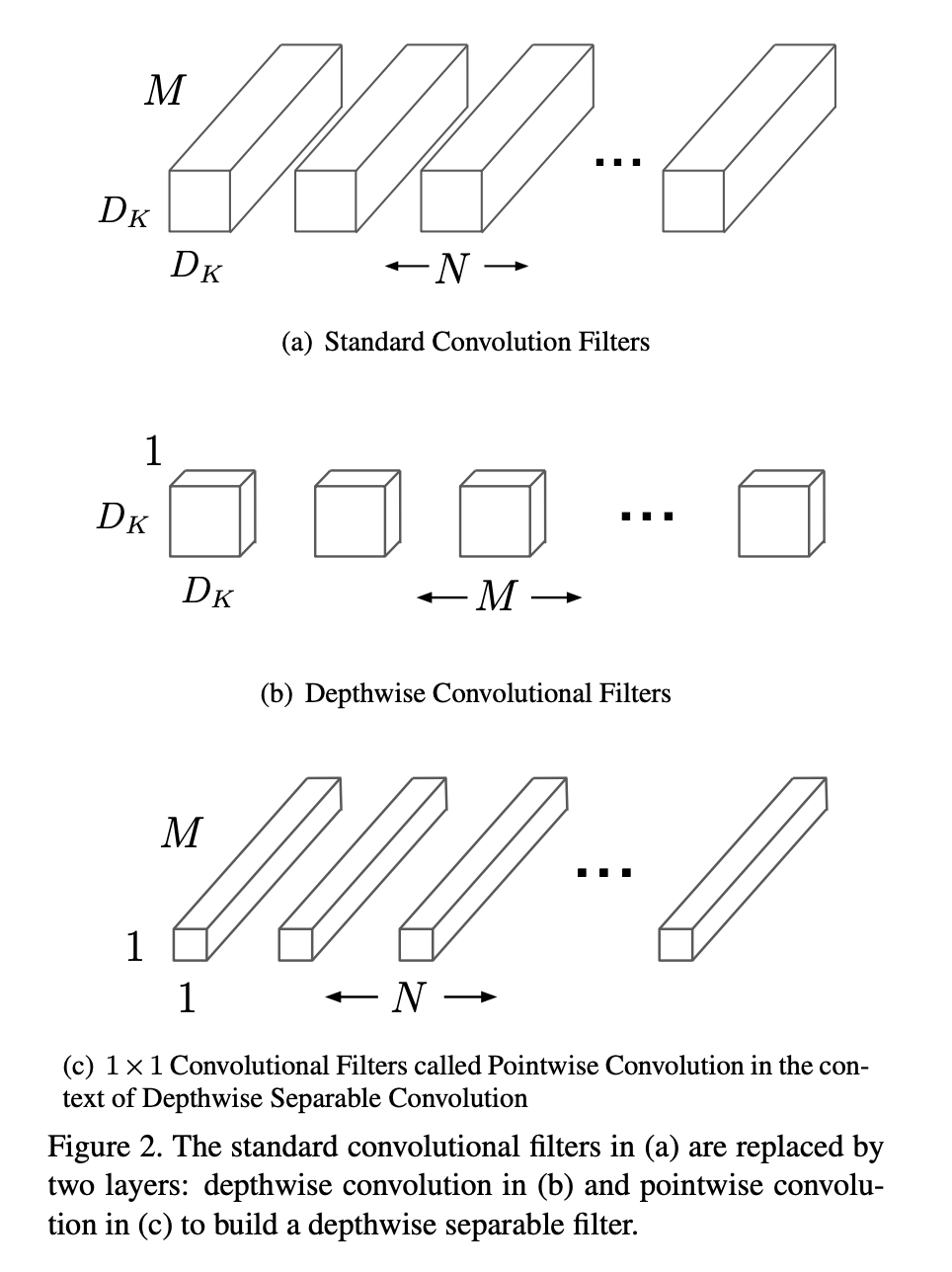
Depth-wise separable convolution and point-wise convolution.

computation cost for standard convolution:

\[\begin{equation} D_K \times D_K \times M \times N \times D_F \times D_F \\ D_F: \text{input feature map size} \\ M: \text{input channels} \\ D_M: \text{filter kernel size} \\ N: \text{filter number or output channels} \end{equation}\]

computation cost for depth-wise separable convolution and \( 1 \times 1 \) point-wise convolution:

\[\begin{equation} D_K \times D_K \times M \times D_F \times D_F + M \times N \times D_F \times D_F \\ \text{first term is for depth-wise separable convolution} \\ \text{second term is for point-wise convolution} \end{equation}\]

the second term takes the bigger part of computation cost.

There are two hyper-parameter of scaling to adjust the model design: width multiplier and resolution multiplier. The role of the width multiplier \( \alpha \) (filter number) is to thin a network uniformly at each layer. The computation cost for these thinner models:

\[\begin{equation} D_K \times D_K \times \alpha M \times D_F \times D_F + \alpha M \times \alpha N \times D_F \times D_F \end{equation}\]

so width multiplier has the effect of reducing computational cost and the number of parameters quadratically by roughly \( \alpha^2 \)

Another hyper-parameter to reduce the computational cost of a neural network is a resolution multiplier \( p \) (input image size),
we apply this to the input image and the internal representation of every layer is subsequently reduced by the same multiplier

\[\begin{equation} D_K \times D_K \times \alpha M \times p D_F \times p D_F + \alpha M \times \alpha N \times p D_F \times p D_F \end{equation}\]

And resolution multiplier has the effect of reducing computational cost and the number of parameters quadratically by roughly \( p^2 \)

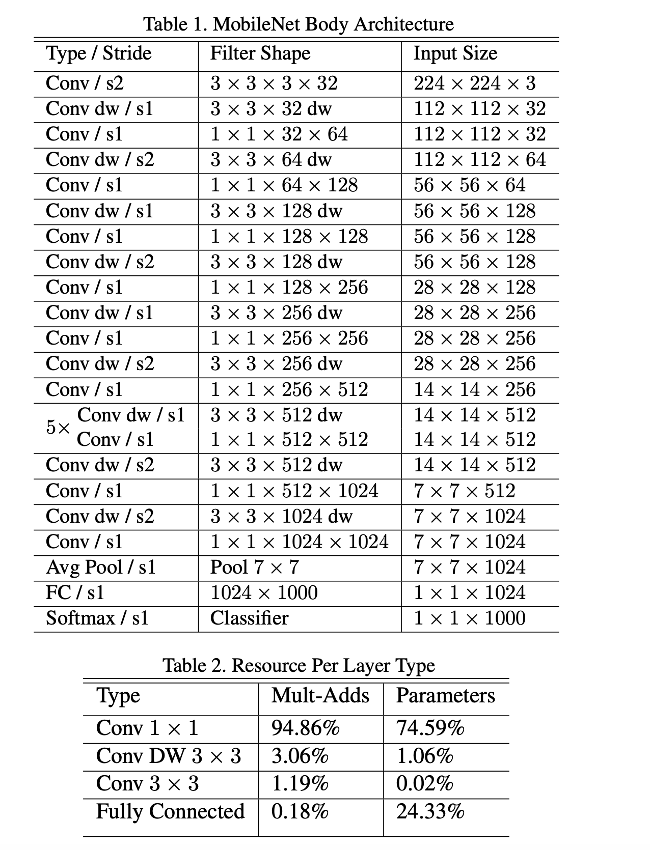
MobileNet structure:

MobileNet body architecture.

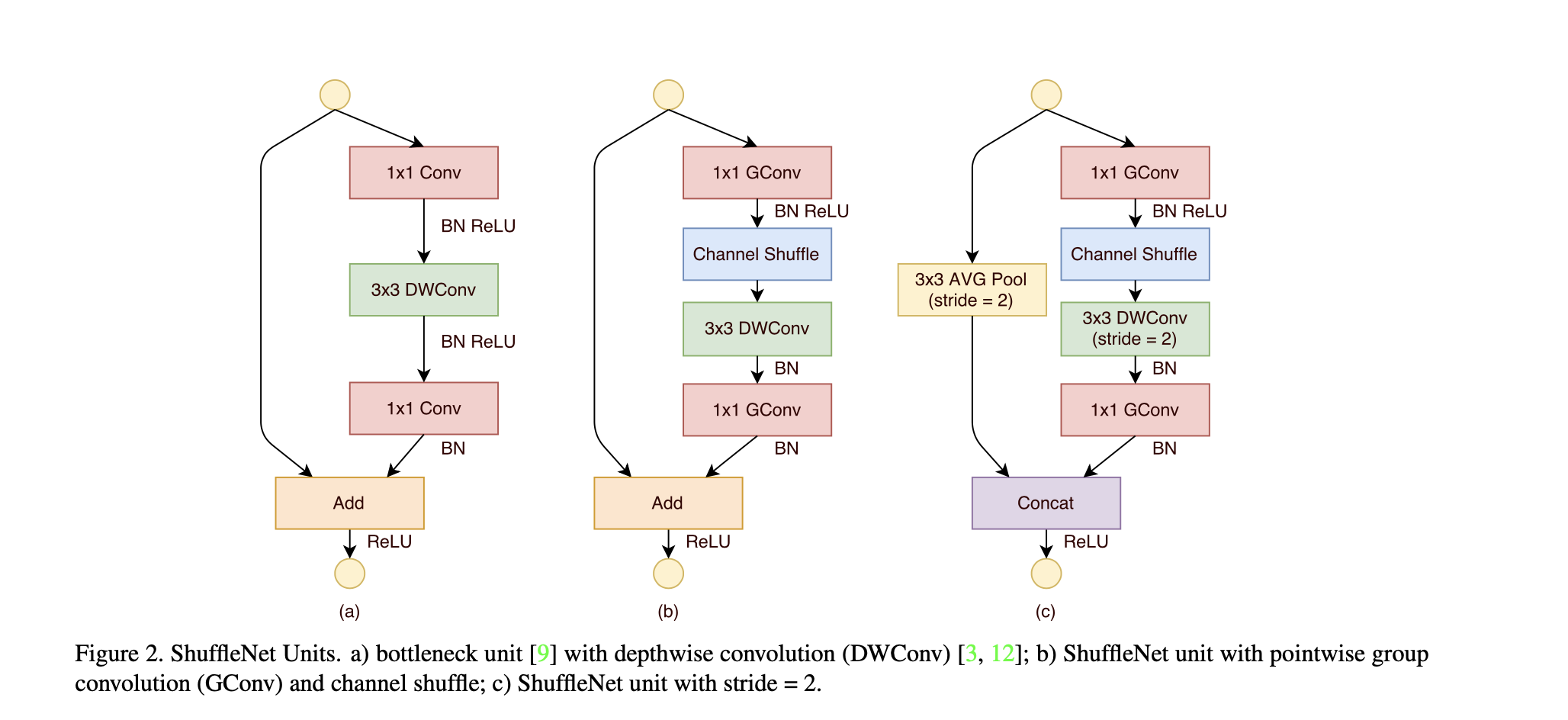
2.ShuffleNet

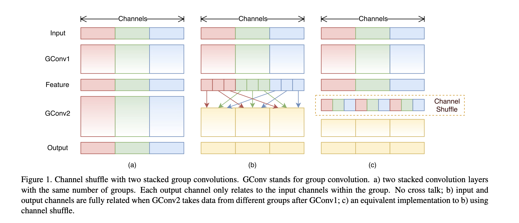
It uses point-wise group convolution and channel shuffle to replace previous \( 1 \times 1 \) point-wise convolution in order to further reduce the computation cost.

The following figure illustrates why the operation of uniform channel shuffle is important. It ensures the communication between different group features after the group convolution.

channel shuffle.

The ShuffleNet unit:

ShuffleNet unit.

3.MobileNetV2

The main contribution is a novel layer module (the inverted residual with linear bottleneck), It takes as an input a low-dimensional compressed representation which is first expanded to high dimension and filtered with a lightweight depthwise convolution. Features are subsequently projected back to a low-dimensional representation with a linear convolution. Another change is to remove non-linearities in the narrow layers to maintain representational power.

inverted residual block: the intermediate layers are thicker. By reducing the number of input and output channels the computation cost could be reduced despite the number of filters in the intermediate layer increases.

inverted residual block.

traditional residual block: the intermediate layers are thinner (from 256 to 64).

residual block.

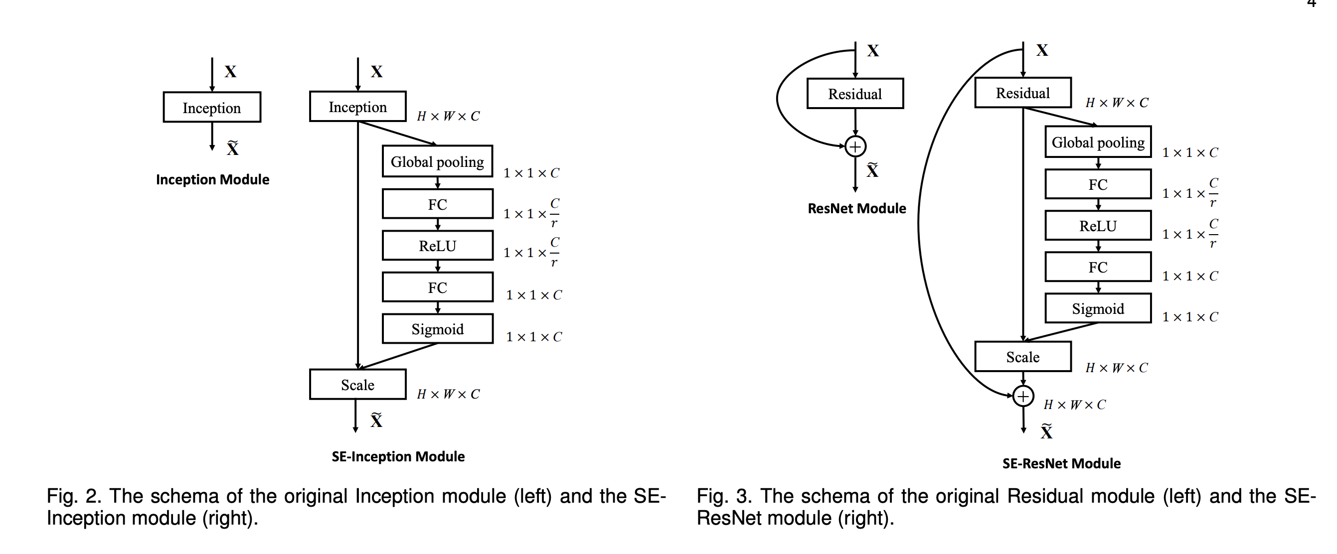
4.SENet

SENet(Squeeze-Excitation-Net): explicitly model the interdependencies between the channels of convolutional features. It is made up of two operations.

squeeze operation: Each of the learned filters operates with a local receptive field and consequently each unit of the transformation output U is unable to exploit contextual information outside of this region, To mitigate this problem, we propose to squeeze global spatial information into a channel descriptor. This is achieved by using global average pooling to generate channel-wise statistics.

excitation operation is to ensure that multiple channels are allowed to be emphasised (rather than enforcing a one-hot activation). To meet these criteria, we opt to employ a simple gating mechanism with a sigmoid activation:

Illustration of Squeeze and Excitation Operation.

The schema of combination between SEBlock and Inception/Residual model is described as following:

Squeeze and Excitation Block.

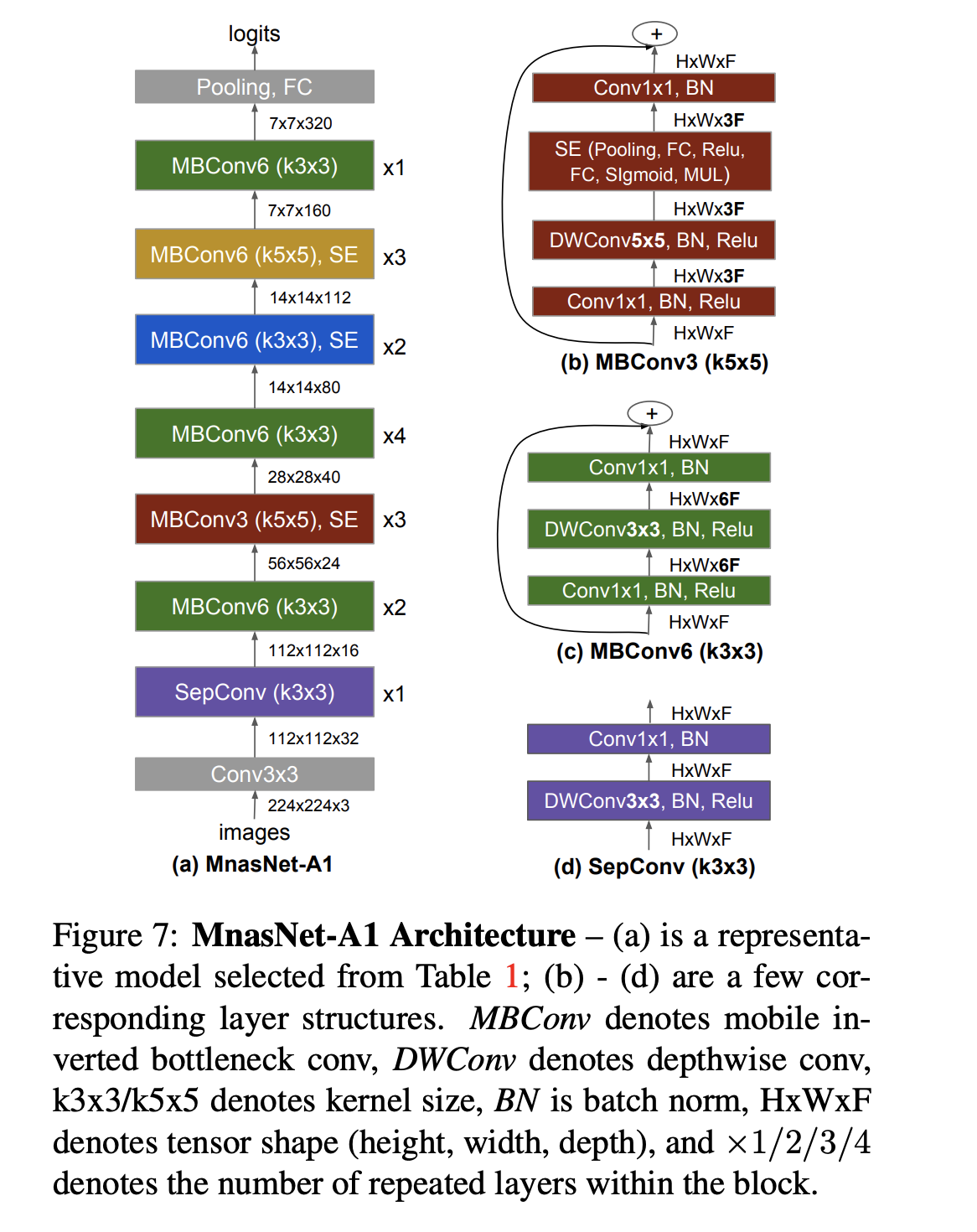
5.MnasNet

It uses automated neural architecture search (NAS) approach for designing mobile models by reinforcement learning. we explicitly incorporate the speed information into the main reward function of the search algorithm, so that the search can identify a model that achieves a good trade-off between accuracy and speed

The overall flow of our approach consists mainly of three components: a RNN-based controller for learning and sampling model architectures, a trainer that builds and trains models to obtain the accuracy, and an inference engine for measuring the model speed on real mobile phones using TensorFlow Lite.

Neural architecture search for mobile.

MnasNet architecture:

MnasNet architecture.

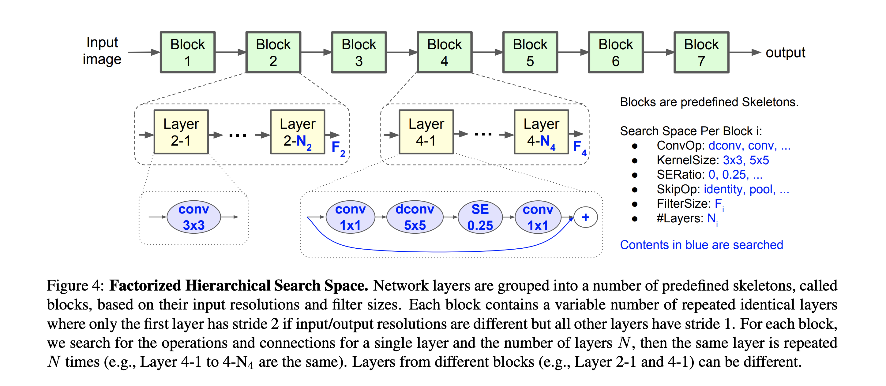
Factorized Hierarchical Search Space: It introduces a novel factorized hierarchical search space that factorizes a CNN model into unique blocks and then searches for the operations and connections per block separately, thus allowing different layer architectures in different blocks. Our intuition is that we need to search for the best operations based on the input and output shapes to obtain better accuracy and latency trade-offs.

Factorized Hierarchical Search Space.

6.EfficientNet

It simultaneously applies compound scaling on width (filter number), depth (layer number), resolution (image size) to find the model architecture with the best efficiency and accuracy.

compound scale on width, depth and resolution.

EfficientNet-B0 architecture is similar to MnasNet but a little bigger. Its main building block is mobile inverted bottleneck MBConv。

EfficientNet-B0 architecture.

EfficientNet-B0 to B7 is acquired as follows:

step 1: we first fix \( \phi = 1 \), assuming twice more resources available, and do a small grid search of \(\alpha, \beta, \gamma\) based on the following equation. In particular, we find the best values for EfficientNet-B0 are \(\alpha = 1.2, \beta = 1.1,\gamma=1.15 \).

\[\begin{equation} depth: d = \alpha^\phi \\ width: w = \beta^\phi \\ resolution: r = \gamma^\phi \\ \quad \quad subject to: \alpha \times \beta^2 \times \gamma^2 = 2 \end{equation}\]

step 2: we then fix \(\alpha, \beta, \gamma\) as constants and scale up baseline network with different \(\phi\), to obtain EfficientNet-B1 to B7

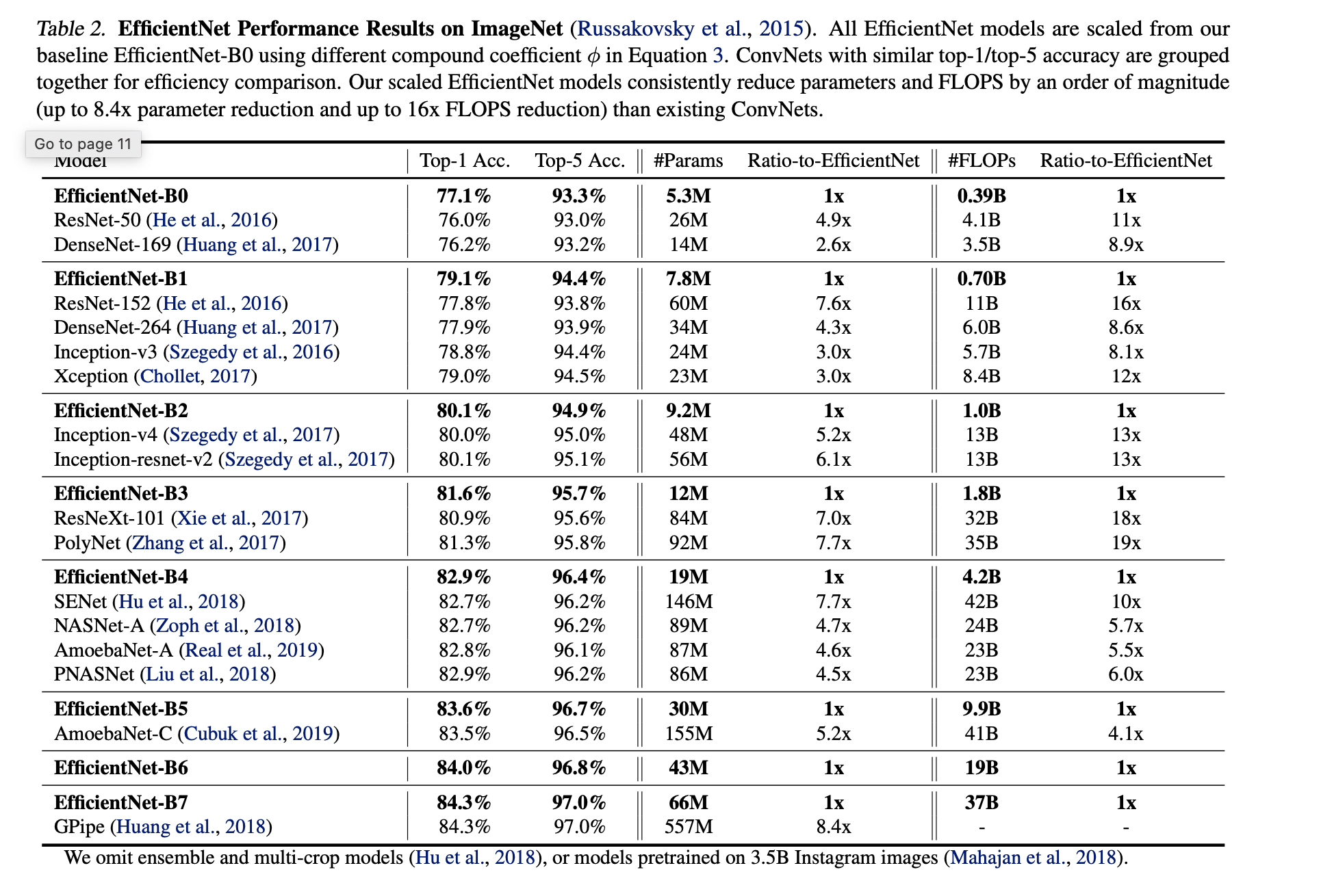
EfficientNet performance on ImageNet:

EfficientNet performance on ImageNet.

compound scaling for MobileNets and ResNet

compound scaling for MobileNets and ResNet.

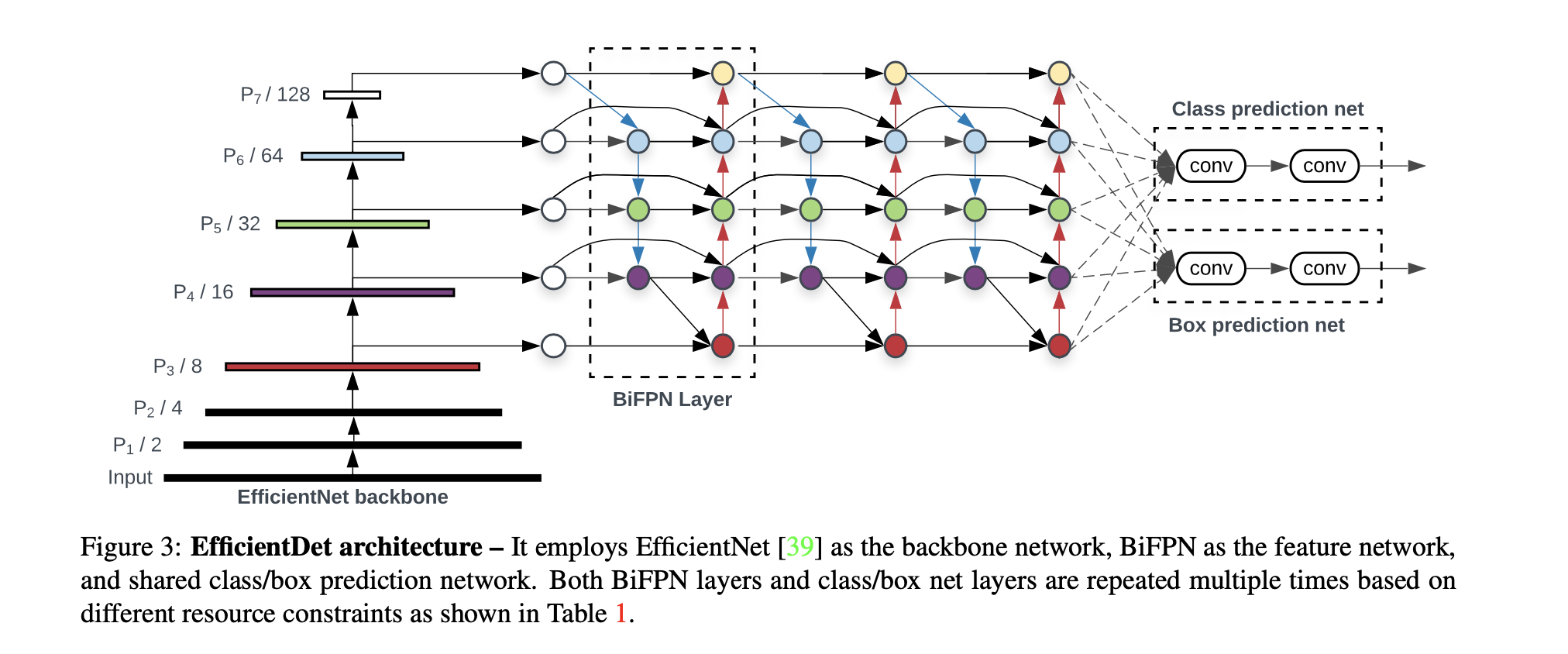
7.EfficientDet

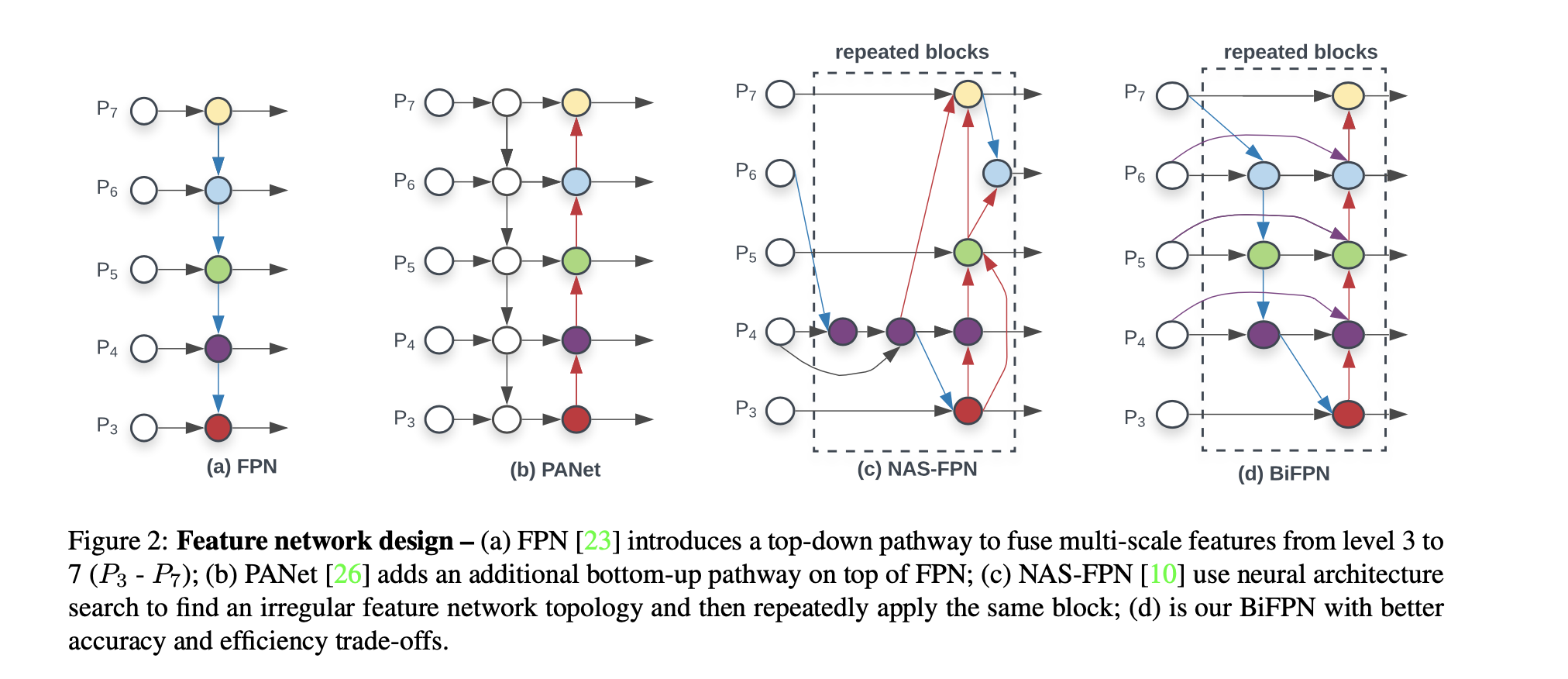
Firstly, it incorporates weighted bi-directional feature pyramid network (BiFPN) without using simple feature pyramid network (FPN), which allows easy and fast multi-scale feature fusion and assigns different weight to the different prediction at the different layer levels.

Secondly, it uses a compound scaling method that uniformly scales the resolution, depth, and width for all backbone, feature network, and box/class prediction networks. This mainly follows the one-stage detector design, and aims to achieve both better efficiency and higher accuracy with optimized network architectures.

Backbone network: reuse the same width/depth scaling coefficients of EfficientNet-B0 to B6 such that we can easily reuse their ImageNet-pretrained checkpoints

BiFPN structure: